Linear real arithmetic

Linear real arithmetic#

This theory follows the shared assignment and explanation contract. Its dedicated arithmetic checks and online callbacks currently provide that integration; the Real routes do not all use the TheoryComponent C++ interface. The interface inventory and combination routes distinguish those paths.

Primo’s linear real arithmetic solver checks whether the inequalities selected by SAT have a common solution. It maintains exact values satisfying a fixed system of linear equations, then repairs violations of the selected bounds. Failure produces a clause explaining which Boolean assignments cannot hold together. The DPLL(T) chapter describes how SAT uses that clause.

The implementation follows Dutertre and de Moura’s Integrating Simplex with DPLL(T), with substantial engineering described below: shared polynomial rows, direct bounds, small-rational arithmetic, sparse pivoting, occurrence indices, deferred checks and bounds-only rollback. Section numbers for this source refer to the technical report, whose numbering differs from the CAV paper.

The integer-arithmetic companion explains how the pure and combined integer routes use this tableau as a real relaxation, then apply patching, GCD checks, Gomory cuts and branching. It covers their explanations, budgets and incomplete cases; its preservation map retains the dated experiments separately.

Theory responsibilities and defaults#

The four main theory operations are collected below. The setup introduces what their bounds and tableau rows represent; each operation then states its input, result, default method and correctness condition.

Operation	Question answered	Default method
Check consistency	Do the currently asserted arithmetic literals have a common solution?	Exact simplex feasibility repair with Sparse pivot selection and eventual Bland fallback.
Explain a theory conflict	Which assertions are inconsistent, and how is their clause obtained?	Two contradictory bounds, or a blocked row of the current tableau and its selected bounds.
Propagate and explain consequences	Which additional registered literals follow from the active bounds?	Same-variable bound propagation; forward and reverse row propagation are off by default.
Construct a model	How does a feasible symbolic assignment become concrete rational values?	Choose a sufficiently small positive rational for the symbolic infinitesimal, then build and reconstruct the typed model.

Conflict detection and explanation are sufficient for the arithmetic consistency decision; theory propagation is an additional search aid. SOI is an optional alternative feasibility procedure. The implementation details also cover pivot policies, sparse storage and theory-combination mechanisms.

Setup and maintained state#

Representation and ownership#

The input to arithmetic preparation is typed core terms plus their Boolean abstraction. The tableau itself receives variable IDs, exact bounds and reason literals. It does not parse SMT-LIB or inspect the SAT solver’s internals.

Representation	Owner, identity and lifetime
LinearPolynomial	Owns a constant and a map from `TermId` to nonzero rational coefficients. Repeated occurrences add; exact cancellation removes an entry.
LraAtom	Owns a normalized polynomial, relation `Le`, `Lt` or `Eq`, and right-hand-side rational. It is a value, not a SAT literal.
PreparedLraTheory	Borrows the term manager and owns the base tableau, term-to-variable map, polynomial-to-slack map, and prepared atom vector. Each atom retains its own threshold and orientation.
LraVarId	A numeric index local to a tableau and its structurally matching copies. It denotes an input leaf or an auxiliary polynomial value, independently of core and SAT IDs.
LraTableau	Owns assignments, bounds with reasons, basic/nonbasic membership, sparse rows, reverse occurrences, violated-variable set and undo records.
OnlineLraPropagator	Borrows prepared data and owns a working tableau copied from the base, decision-level checkpoints, pending consequences and retained reasons. It reads the shared SAT assignment view.

The term manager must outlive preparation and any interpretation of its IDs. Tableau IDs survive pivots and rollback; being basic is a mutable property of the variable. Structural insertion allocates vectors and maps, and pivots can replace entire rows. References into these containers must not survive such mutations. Copying a tableau preserves its numbering but creates independent mutable arithmetic state.

The usual preparation installs equations before search. append_atom can extend the prepared base between SAT calls, for example for a new interface equality. This is separate from asserting a bound on the live tableau; add_row is not a trailed search operation.

Tableau equations and bounds#

The tableau partitions its variables into basic variables, each defined by a row, and nonbasic variables, whose values can be chosen independently before recomputing the basic values. A row has the form

\[ x_b=\sum_{j\in N}a_{bj}x_j, \]

where \(N\) is the nonbasic set and every coefficient \(a_{bj}\) is rational. Write \(\beta(x)\) for the current assignment and \(l(x),u(x)\) for the active lower and upper bounds when present. Bounds and assignments use delta rationals. Each bound carries the negation of its asserting SAT literal as its reason; those reasons will identify the premises of a conflict or propagation clause.

The equations are identities introduced by arithmetic preparation. Pivoting solves one row for a different variable and substitutes that equation into the other rows. It changes the basis while preserving the represented system. The linked LraTableau owns these rows, values and bound reasons; the sparse representation describes their storage and update costs.

From atoms to bounds#

LinearPolynomial::from_term collects additions and constant scaling. Core Times stores a rational coefficient and one child, so it represents linear scaling. Arithmetic leaves are identified by their TermId; any uninterpreted application needs the surrounding combination machinery to enforce its function semantics. Unlowered ite, div, mod and abs raise an exception at this boundary.

normalize_atom subtracts the right side and moves the constant to the threshold. Preparation then orders variables by TermId and divides every coefficient and the threshold by the first coefficient, making that coefficient one. A negative divisor reverses the inequality. This canonicalization identifies proportional polynomials; it does not merge their SAT variables.

For example, these predicates can share the variable s = x + y:

Predicate	Bound when true
`x + y <= 5`	`s <= 5`
`2x + 2y <= 10`	`s <= 5`
`-x - y <= -5`	`s >= 5`
`x + y <= 7`	`s <= 7`

The thresholds and SAT reasons stay separate, including when a predicate is assigned false. A single-variable polynomial instead becomes a direct bound: 2*x <= 10 needs x <= 5, with no auxiliary variable or equation. PreparedLraTheory::append_atom implements both savings: bounds on a single variable use that variable directly, while bounds on proportional compound polynomials share one auxiliary variable and its defining row. This keeps the tableau smaller and puts related bounds on the same variable, where they can be compared directly.

Monniaux’s CAV 2009 paper, §2.1, describes both ideas, but chooses a different standard form for the coefficients. The paper clears denominators and removes common integer factors, choosing the sign so the first coefficient is positive. Primo divides by the first coefficient, so it becomes exactly one; the remaining coefficients may be fractions. For example, assuming x comes before y in the variable order:

Input	Paper’s integer form	Primo’s form
`4x + 6y <= 10`	`2x + 3y <= 5`	`x + (3/2)*y <= 5/2`

The paper’s coefficients 2 and 3 have greatest common divisor one: this is what “coprime integer coefficients” means here. Both forms express the same inequality and give proportional polynomials a common representation. In both cases the threshold must be scaled by the same factor as the coefficients.

Leading-coefficient normalization gives Primo a simple way to share rows. canonical_polynomial uses one coefficient as the divisor for every term and the threshold, skipping those divisions when it is already one. It needs no separate common-denominator or greatest-common-divisor computation across the vector; individual rational operations still reduce their results.

The tradeoff is that this can introduce fractions into an initially integer row. Coprime-integer normalization avoids those initial fractions, but clearing input denominators can enlarge coefficients, and later pivots can introduce fractions again. There is no recorded direct performance comparison of the two normal forms; the normalization review records the original row-sharing objective and available evidence. Choosing an initial normal form and maintaining integer rows throughout pivoting are separate design questions.

Primo also has a separate, optional early atom canonicalizer that uses coprime integer coefficients in core terms, so equivalent predicates can share a SAT atom. It is off by default. Even when enabled, tableau preparation still applies leading-coefficient division. The early canonicalization note describes that separate transformation and its evaluation.

Real equality is lowered to two inequalities before this path. Negating it gives a Boolean choice between strict inequalities, handled by SAT. The low-level Eq case’s rejection of a false equality is therefore not a restriction on surface Real disequality. See the equality-lowering design and bound assertion boundary.

Exact numbers and strict bounds#

util::Rational uses an inline signed 64-bit numerator and denominator for values fitting its small representation. Operations use checked wide intermediates and fall back to GMP rationals. Results that fit return to the small representation: equal values must compare and hash alike regardless of the arithmetic path that produced them. This is the two-tier representation discussed by Monniaux §4 and Griggio §2.5.2, with 64-bit rather than Monniaux’s 32-bit small values. The paper’s floating-point solver and forced-pivoting algorithm remain an open lead: floating-point-guided basis selection.

The compact rational storage lead investigates overlapping the small numerator and owned big-number pointer. It includes a reproducible layout probe and the remaining ownership and evaluation questions.

A strict bound uses an exact symbolic infinitesimal. DeltaRational stores two rationals (q, k), interpreted as q + k*δ, ordered lexicographically. The rational part is compared first; the infinitesimal part breaks ties. Thus \(0<\delta<r\) for every positive rational \(r\), and \(2-\delta<2<2+\delta\). There is no floating-point tolerance. For an unflipped Real atom:

Atom	Assigned true	Assigned false
`t <= c`	upper bound `(c, 0)`	lower bound `(c, 1)`
`t < c`	upper bound `(c, -1)`	lower bound `(c, 0)`

The flipped orientation reverses the bound direction. All cases are centralized in bound_assertion. Integer tightening is a separate branch of this function; the infinitesimal interpretation here is for Real arithmetic. The basis is Dutertre–de Moura §3.3, including the argument that a sufficiently small positive rational can replace δ in a satisfying model.

Check consistency#

Contract	Meaning
Input	The prepared tableau equations, plus currently asserted bounds with their reason literals.
Result	A successful `check()` returns no conflict; a failed bound assertion or check returns an owned vector of SAT clause literals.
Default method	Ordinary feasibility repair with Sparse pivot selection and eventual Bland fallback.
Correctness condition	Success means one assignment satisfies every tableau equation and active bound. Failure must be justified by an inconsistent subset of asserted bounds.

Feasibility without an optimization objective#

Proving UNSAT with delta rationals does not require optimizing \(\delta\) or introducing an objective function. The ordinary repair procedure checks feasibility: whether the tableau equations and active bounds have a common solution in the lexicographically ordered pairs. Dutertre–de Moura §3.3 shows that this encoding preserves satisfiability for finite systems of rational linear constraints with strict inequalities. Consequently, a contradiction in the encoded system proves that the original constraints are unsatisfiable.

During this check, \(\delta\) stays symbolic. Choosing a sufficiently small positive rational to replace it belongs to constructing a satisfying model, after feasibility has been established; an UNSAT proof needs no such choice.

Repairing an assignment#

Dutertre–de Moura §3.2 separates three obligations:

Every assignment satisfies the tableau equations.
Every nonbasic variable satisfies its current bounds.
After a successful check(), basic variables satisfy their bounds too.

assert_upper and assert_lower tighten a bound and save its predecessor on the undo trail. A weaker bound does nothing. A new upper bound below the current lower bound, or conversely, returns an immediate conflict without installing the contradictory bound. If a nonbasic value falls outside a new bound, update moves it to that bound and updates dependent basic values. Basic variables may then need repair.

For the ordinary repair policies, check selects a violated basic variable and a nonbasic variable that can move in the required direction. It pivots the latter into the basis, then moves the now-nonbasic leaving variable to its violated bound. For example, pivoting y into the row s = x + y yields y = s - x; setting s to its target updates y and every other row depending on s. Each pivot preserves the equations. If no eligible entering variable exists, current bounds prevent repairing that row, and the solver explains a conflict.

The solver selects Sparse by default and eventually uses Bland to ensure termination; a directly constructed LraTableau defaults to Bland. The policy details describe the choices and fallback threshold. If no basic variable remains violated, check() succeeds. If a row is blocked, conflict explanation identifies the assertions responsible. The complete rational feasibility procedure can therefore decide inconsistency without enabling theory propagation or SOI. This completeness claim concerns linear real arithmetic; the integer relaxation needs additional integer reasoning.

Deferred consistency checks#

The online propagator applies each assigned bound immediately but defers simplex repair until a consistency check is needed. This batches check() calls, not the bound updates themselves; deferred assignment updates remain a different proposal. An immediate bound conflict must survive the deferred check because the rejected bound never entered the tableau. See notification and deferred repair. Delivered propagation reasons remain available until their assignments are removed, following the shared-assignment protocol in DPLL(T).

Explain theory conflicts#

Contract	Meaning
Input	Either two contradictory bounds on one variable, or a violated basic row for which no eligible repair variable exists.
Result	A clause containing the negations of the asserting SAT literals for the conflicting bounds.
Default method	Direct bound comparison, followed when necessary by a single-row explanation after feasibility pivots.
Correctness condition	The selected assertions and tableau identities imply a contradiction. Their negations therefore form a theory-valid clause.

These are explanations of theory conflicts. A propagation explanation instead justifies an additional literal and is covered in propagation. The ordinary conflict procedure follows Dutertre–de Moura §3.2.2.

Directly contradictory bounds#

If assertions p and q impose \(x\ge l\) and \(x\le u\) with \(u<l\), assert_upper or assert_lower returns the existing bound’s reason and the incoming bound’s reason, forming \(\neg p\lor\neg q\). The comparison is exact, including infinitesimal parts. The rejected bound need not be installed and no pivot is required; the bound assertion operations handle this case.

Selecting bounds from a blocked row#

Consider a current basic row \(x_b=\sum_j a_jx_j\). If \(\beta(x_b)<l(x_b)\) and no nonbasic variable can move to increase \(x_b\), the positive-coefficient variables are at their upper bounds and the negative-coefficient variables are at their lower bounds. These bounds imply

\[ x_b\le U=\sum_{a_j>0}a_j u(x_j)+\sum_{a_j<0}a_j l(x_j) =\beta(x_b)<l(x_b). \]

The explanation selects the violated lower bound on \(x_b\) and each bound used in \(U\). For a variable above its upper bound, the symmetric calculation is

\[ x_b\ge L=\sum_{a_j>0}a_j l(x_j)+\sum_{a_j<0}a_j u(x_j) =\beta(x_b)>u(x_b). \]

Here the explanation selects the violated upper bound and the bounds used in \(L\). Every selected bound exists: an absent blocking bound would leave an eligible movement direction. The entering-variable selection establishes that the row is blocked, and build_conflict selects the corresponding reasons according to coefficient signs. The row identity needs no SAT premise. Collecting its selected bound reasons forms the conflict clause; the mathematical inequalities explain why that clause is valid.

Minimization and alternative explanations#

The default single-row procedure has no separate minimization pass. It uses the current blocking bounds, with one active bound per direction on each variable; it does not search weaker sufficient bounds or expand shared propagation antecedents. SAT can resolve propagated literals through their reasons during conflict analysis. Its final learned clause can differ from the theory explanation.

A derived numeric bound need not have a SAT naming literal. If used to explain a conflict, its internal proof must first be expanded to SAT-visible premises by the theory. Compatible assigned stronger bounds do tighten the tableau: the new value and its asserting literal’s reason replace the previous pair; an immediately contradictory bound returns a conflict instead. For a propagated literal, the SMT callback separately retains its antecedents for SAT analysis; see the worked tightening explanation. Current row propagation returns derived values with those premise reasons and proves registered atoms; it does not install a general graph of internal derived bounds. The survey distinguishes these cases from temporary bounds in private equality probes.

The optional SOI minimizer reduces selected violated rows. It is separate from arithmetic bound weakening and from SAT learned-clause minimization. Classical SAT minimization deletes literals; all-UIP shrinking can introduce replacement antecedents. King’s thesis §2.2.9 describes another choice: weaken bound premises while preserving the numerical contradiction. These distinctions, current implementation limits and worked examples are in the literature survey and proposed probe.

Why one current row suffices after pivoting#

A current tableau row can combine several original equations. For example, let SAT assert all three literals

p: x + y <= -1       q: x - y <= -1       r: x >= 0

Introduce basic variables \(s_1=x+y\) and \(s_2=x-y\), carrying upper bounds \(s_1\le-1\) from p and \(s_2\le-1\) from q. Initially set \(x=y=0\); both basic variables violate their upper bounds. Each row can be repaired individually by moving \(y\) while keeping \(x\ge0\).

One possible feasibility pivot repairs \(s_1\) using \(y\). Solving the first row and substituting into the second gives

\[ y=s_1-x,\qquad s_2=x-(s_1-x)=2x-s_1. \]

Setting the now-nonbasic \(s_1=-1\) gives \(y=-1\) and \(s_2=1\) when \(x=0\). The single current row for \(s_2\) is now blocked: decreasing \(x\) is prevented by \(x\ge0\), and increasing \(s_1\) is prevented by \(s_1\le-1\). Its selected bounds imply

\[ s_2=2x-s_1\ge2\cdot0-(-1)=1, \qquad s_2\le-1, \]

a contradiction explained by \(\neg p\lor\neg q\lor\neg r\). This is an illustrative pivot sequence; the selection policy can choose another sequence leading to a conflict. The pivot operation maintains the substituted identities, so the final explanation needs only the current row and its bounds. A single original constraint need not already expose the contradiction. SOI can also combine these two rows directly, but is not required to explain it.

Follow a strict conflict#

Let SAT assign p, q and r true for:

p: x + y <= 2       q: x >= 2       r: y > 0

Preparation supplies s = x + y, initially with all values zero. The following is a trace of theory operations, not a prescribed SAT search order:

Operation	Assignment and bounds
Assert `p`	Install `s <= 2`, carrying reason `¬p`.
Assert `q`	Install `x >= 2`, carrying `¬q`; update `x = 2`, hence `s = 2`.
Assert `r`	Install `y >= δ`, carrying `¬r`; update `y = δ`, hence `s = 2 + δ`.
Check the violated row	`s` is too high. Decreasing either `x` or `y` is blocked by its lower bound, so no repair pivot is possible.

The row and the two lower bounds imply s >= 2 + δ, contradicting s <= 2. The resulting clause is ¬p ∨ ¬q ∨ ¬r.

The same contradiction can be checked by rewriting the three encoded bounds with \(\le\) and adding them:

\[\begin{split} \begin{aligned} x+y &\le 2,\\ -x &\le -2,\\ -y &\le -\delta \end{aligned} \qquad\Longrightarrow\qquad 0\le-\delta. \end{split}\]

The variables cancel, and the last inequality is false because \(-\delta=(0,-1)<(0,0)=0\). All three weights in this combination are the nonnegative rational \(1\), so adding the inequalities preserves their direction. More generally, nonnegative rational combinations of inequalities can certify a conflict when all variable coefficients cancel and the right-hand side is negative in the delta ordering. This explains the mathematical proof; it does not imply that Primo exports those weights.

Primo stores the negation of the asserting SAT literal with each bound, at the assignment boundary. build_conflict collects the violated bound’s reason and the row bounds that block movement. It returns clause literals directly; the caller must not negate them again. This is the row-based explanation of Dutertre–de Moura §3.2.2. The returned object is a SAT clause, not an exported proof certificate with coefficients.

This clause excludes the current combination of arithmetic assertions. For a Boolean combination of constraints, SAT uses such clauses to continue the search; one arithmetic conflict alone need not make the whole formula UNSAT. See the DPLL(T) chapter.

The optional sum of infeasibilities mode uses an objective to guide repair. A zero sum means all bounds hold; a proven positive minimum establishes infeasibility. A positive violation at an arbitrary assignment does not suffice. This objective is a search method, not a requirement imposed by delta rationals, and \(\delta\) itself is never the optimization variable.

Propagate and explain consequences#

Contract	Meaning
Input	Active bounds with reasons, tableau equations, and registered arithmetic atoms with SAT names.
Result	An implied SAT literal and a clause consisting of that literal and the negated premises. No consequence is also a valid result.
Default method	Compare bounds on the same variable. Forward and reverse row propagation require their separate options.
Correctness condition	The asserted premises imply the propagated literal. Discovery of all consequences is not required.

Arithmetic propagation proves the value of an existing Boolean atom from active bounds and the tableau equations. It returns that literal with an explanation clause. Equality exchange uses the same implication-to-clause principle to communicate consequences between theories; its conclusions are equalities of shared terms.

Bounds on the same variable#

Default propagation compares predicates bounding the same tableau variable. For instance, p: s <= 2 entails t: s <= 5, with reason clause ¬p ∨ t. scan_for_propagations visits the prepared atoms_by_bound_var index and checks both polarities of each unassigned atom. It uses bounds, not accidental equalities in the current candidate assignment. This is the cheap propagation of the technical report’s §3.2.5.

Deriving a bound from a row#

Optional row propagation combines bounds on several variables. Consider the current tableau row

s = 2*x - 3*y + z

Here s is basic and x, y, z are nonbasic; the equation is an identity maintained by pivoting, not an extra SAT assumption. Let l(v) and u(v) denote the active lower and upper bounds on variable v. Multiplication by a negative coefficient reverses order, so the bound used for each contribution depends on its sign:

Coefficient of `v`	Upper-bound contribution	Lower-bound contribution
`a > 0`	`a*u(v)`	`a*l(v)`
`a < 0`	`a*l(v)`	`a*u(v)`

Thus this row gives

upper(s) = 2*u(x) - 3*l(y) + u(z)
lower(s) = 2*l(x) - 3*u(y) + l(z)

These are candidate implied bounds; they need not be the strongest bounds entailed by the whole problem. compute_implied_bound computes one direction at a time with exact DeltaRational arithmetic and collects the reasons of the selected bounds. It reads bounds, not the current model’s values of x, y and z.

For a concrete upper bound, suppose SAT literals p, q, r assert x <= 4, y >= 1, z <= 2. The contributions are at most 8, −3 and 2, respectively, so s <= 7. If an unassigned atom has literal t and means s <= 8, this entails t with the clause

not p or not q or not r or t

The threshold may be weaker than the computed bound: 7 <= 8 suffices. For a lower-bound query the comparison reverses. The entailment check makes this comparison against the bound imposed by each possible truth value of the target atom. It can therefore propagate the negation of an atom as well.

The same calculation handles strict bounds using the infinitesimal convention. Replacing x <= 4 by x < 4 contributes 2*(4 - δ) and gives s <= 7 - 2*δ. This is strong enough to imply the atom s < 7, whose upper bound is 7 - δ.

Bounding a row variable in reverse#

The optional reverse direction isolates a nonbasic variable rather than the row’s basic variable. In a separate candidate with the same row, let literals a, b, c assert s <= 1, x >= 2, z >= 0. Isolating y gives

-3*y = s - 2*x - z <= 1 - 2*2 - 0 = -3
   y >= 1

Dividing by −3 reverses the inequality. If literal v represents the unassigned atom y >= 1, its explanation is not a or not b or not c or v. This derivation uses the bound on s and the other row variables; it does not need an existing bound on y.

In general, for s = k*y + sum(k_j*x_j) with nonzero k, isolate y = (s - sum(k_j*x_j))/k. Choose the numerator’s upper or lower bound according to the requested direction and the sign of k, then apply the coefficient rule above to the subtracted terms. This is compute_implied_child_bound. It returns a derived value and the clause literals explaining the selected bounds, without pivoting to make y basic.

Delivery, triggers and limits#

Both helpers retain the bounds’ already negated premise literals: the forward example stores not p, not q, not r. The delivery and reason callbacks return the target literal and these clause literals without negating them again. The propagator owns the queued candidates and delivered reasons, following the explanation lifetime rules. A row identity needs no SAT premise; changing basis does not invalidate the identity used to derive the clause.

The implementation uses derived bounds to test already registered atoms. It does not install every derived numeric bound or iterate interval refinement to a fixed point. Only when SAT assigns a propagated atom does its bound enter the usual assignment path and become available for further propagation. In the forward example, deriving s <= 7 proves the existing atom s <= 8. Assigning that atom submits the bound 8 to the tableau, not the derived bound 7; an already stronger stored bound remains in force.

After a nonconflicting assigned bound, the notification hook invokes the optional row scan. scan_row_based_propagations follows occurs_in(changed_var) to rows containing the changed variable. It skips rows without indexed atoms on their basic variable; otherwise it tests those atoms and, when enabled, runs the reverse scan over atoms on the other row variables. This is selective scheduling: a change to a basic variable’s own bound alone does not visit its defining row through occurs_in. In the reverse example, a subsequent bound notification for x or z can trigger the calculation once the needed bounds are present. Pivots do not themselves run this scan.

Missing bounds and cost caps can prevent a propagation without changing satisfiability. Without a lower bound on y, the forward example cannot compute its upper bound by this interval calculation; another direction or another row may still yield a consequence. A row wider than the size cap is skipped. If the changed variable occurs in more rows than the fanout cap, the scan skips all of them for that notification rather than taking a prefix. The default caps are 64 terms/rows for forward work and 32 for reverse work. Each target-atom query can rescan the row, so the cost also depends on how many atoms index the affected variables.

The options enable same-variable propagation by default; row propagation requires lra_row_propagation, and the reverse direction additionally requires lra_bidirectional_row_propagation. Both row options default to false and depend on lra_propagation. These mechanisms do not perform complete arithmetic consequence discovery.

Dutertre–de Moura’s technical report §3.2.5 describes both same-variable propagation and row-bound refinement; applying it to an isolated row variable gives the reverse rule above. Primo’s atom indexing, triggers and caps are implementation choices. Bjørner and Nachmanson’s Arithmetic Solving in Z3 (CAV 2024), §3.3, makes the same direct/indirect propagation distinction. Primo’s row mode queries implied bounds to explain existing Boolean atoms; this does not mean it implements every bound-refinement policy described for Z3.

For mixed Real problems, a proved comparison can also contribute to online shared-equality propagation: assigned x <= y and y <= x justify x = y. The default tableau equality rules are another producer, with their own scheduling and completeness limits. These are separate from guessing an equality because two current model values happen to coincide.

Model construction#

Contract	Meaning
Input	A feasible tableau for the accepted arithmetic assignment, prepared term-to-variable mappings, and model reconstruction information.
Result	Concrete rational values incorporated into the typed model.
Default method	Instantiate the symbolic infinitesimal with a sufficiently small positive rational and reconstruct the model.
Correctness condition	All selected arithmetic literals remain true; tableau equations and required shared-value relationships are preserved.

From delta rationals to rational values#

For a satisfying Real model, choose_concrete_delta finds a positive rational small enough to preserve the assigned bounds and evaluates q + k*δ at that value. Where a crossing point limits δ, it chooses half the smallest positive limit; otherwise it uses one. Mixed theory model construction additionally preserves required shared-value orders. Reconstruction of eliminated variables and Boolean values remains part of the model builder; a feasible tableau alone is not the printed model.

For example, \(x>2\) and \(x\le3\) can have the symbolic assignment \(x=2+\delta\). Preserving its encoded upper bound requires \(\delta\le1\). The crossing limit is \(1\), so the choice \(\delta=1/2\) yields \(x=5/2\), which satisfies both original inequalities. Each variable uses the same chosen value of \(\delta\), preserving rational linear equations.

The Real model construction path uses real_model_values_from_lra to map prepared term IDs to concrete values and build_qf_lra_model to pass those values, Boolean atom assignments and model conversions to the typed model builder. These values are an output assignment, not new entailed bounds. For mixed theories, model reconciliation also has to agree on shared values.

Incrementality and rollback#

push() returns an undo-trail position. With the default sparse policy, pop restores bounds and rebuilds the set of violated basic variables. It retains the current basis and assignment. Relaxing bounds preserves nonbasic feasibility, and the assignment still satisfies the retained equations. Basic feasibility is established by check(), not by the act of popping alone.

This is an implementation choice within the fixed-equation approach. The technical report §3.2.4 describes saving a successful assignment; Bromberger §7.1.3 compares that with keeping the current assignment and rechecking. Primo neither restores an old assignment against a changed basis nor unconditionally runs check() inside pop(). SAT decision rollback and SMT-LIB assertion scopes remain different operations. The latter’s reuse design is described in the retained LRA session note.

The SOI objective depends on which basic variables currently violate which bounds. Restoring bounds alone would leave its cached directions and row describing the abandoned state. Primo therefore trails assignments, pivoted rows, and objective changes in SOI mode, as selected by trails_assignments_and_pivots. Each FRowTrailEntry saves the previous objective row together with the changed variable’s previous direction. Undo restores both, and pop rebuilds the occurrence index after row restoration and the violated-variable set after all undo operations. This is Primo’s current restoration strategy; an alternative could recompute the objective from the retained basis and restored bounds.

Optional algorithms and implementation details#

The sections above describe the standard theory operations. The following sections give optional alternatives, storage and selection details, and the additional mechanisms used for theory combination. Each states its own defaults and scope.

Pivot-selection policies#

The solver’s default is Sparse, although a directly constructed LraTableau defaults to Bland. The solver options select the policy:

Policy	Implemented choice
Default sparse leaving	Shortest violated row; greatest violation breaks ties.
Sparse entering	Fewest column occurrences among eligible candidates considered; unit coefficient, then variable ID break ties. By default, compare at most 16 eligible candidates. The scan may visit more entries to find them.
Optional least-violated leaving	Griggio §2.5.3: smallest violation first, then shortest row. This overrides the default leaving policy under Sparse.
Optional Dantzig	Greatest violation first; largest absolute entering coefficient, with variable IDs breaking ties.
Bland	Smallest eligible variable IDs on both sides; also the termination fallback.
Optional SOI	Maintains a joint objective for all current violations; see sum of infeasibilities.

Monniaux §3 also describes preferring shorter rows and fewer column occurrences to reduce pivot cost, in the context of forced pivoting. Primo’s sparse policy applies that rationale to ordinary feasibility search; it does not import the surrounding floating-point/forced-pivot procedure. King §2.2.12 provides the direct comparison for minimum-column selection and eventual Bland fallback in SMT.

Heuristic selection eventually switches to Bland within each check() call. The default threshold is 4 * variable_count + 64; this is a tuning choice, not a bound on the total pivots needed. King §2.2.12 explains why eventual Bland selection matters. The selection scan must still find an eligible candidate beyond an unproductive row prefix; otherwise a cost cap could become an incorrect conflict. See select_entering_variable.

Sparse rows and reverse occurrences#

The tableau stores each basic row as a sorted vector of nonzero coefficients, with one entry per nonbasic variable. The actual entry is RowEntry {var, coeff, occ_slot}. Its reverse link satisfies:

For entry e in rows_[b]:  occurs_in_[e.var][e.occ_slot] == b

occurs_in_[v] lists the basic rows containing v. Its order is immaterial. occ_slot locates the column occurrence, not the row entry. Removing an occurrence swaps the last column element into its place and repairs that element’s row backlink using binary search. Thus unlink_occurrence avoids scanning the column, but repair is logarithmic in the moved row’s length. It is not the constant-time unlink of a doubly linked matrix.

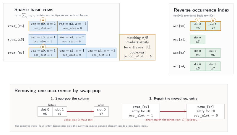
Sorted tableau rows linked by occ_slot to unordered column occurrence lists, with swap-pop removal and backlink repair. — Fig. 3 Sorted rows and their reverse occurrence index. Each row entry’s `occ_slot` locates its entry in a column list; `occ` abbreviates `occurs_in_`. The editable TikZ source is retained with the figure.#

The distinction among the thesis representations matters. King §2.2.7 uses unsorted, doubly linked rows and columns, with a dense scratch map for row addition. Griggio §2.5.2 discusses sorted contiguous coefficient arrays. Bromberger §7.1.4 uses sorted doubly linked rows, unordered columns and a common denominator per row. Primo uses sorted vectors, individual rational coefficients and the indexed occurrences above. These designs support the same sparse operations with different allocation and removal costs.

pivot merges sorted rows, drops exact cancellations and updates occurrences only when membership changes. The coefficient merge is linear in the two row lengths; occurrence repairs and arbitrary-precision arithmetic add their own costs. Updating a nonbasic assignment visits its dependent rows through occurs_in_, but the current update still searches each affected row for the coefficient. The occurrence index is not a direct pointer to that coefficient. The column-to-row coefficient lead lists every such lookup and the candidate representations.

The 32-bit occurrence slot assumes fewer than 2^32 occurrences in a column. The representation and its capacity assumption are distinct from SAT literal encoding. Hash-consing core terms does not bound either quantity.

Optional sum of infeasibilities#

--lra-pivoting-rule soi selects sum of infeasibilities (SOI). This mode uses all current bound violations to guide a repair step. The ordinary sparse policy remains the solver default. The algorithmic basis is King, Barrett and Dutertre’s Simplex with Sum of Infeasibilities for SMT, FMCAD 2013, §V, and King’s thesis, §§3.2–3.3. The implementation choices and departures are described below.

The violation objective and its row#

Write \(\beta(x)\) for the current exact assignment, and \(l(x)\) and \(u(x)\) for the active bounds when present. Define the violation of a variable by

\[\begin{split} v_\beta(x)= \begin{cases} l(x)-\beta(x), & \beta(x)<l(x),\\ \beta(x)-u(x), & \beta(x)>u(x),\\ 0, & \text{otherwise}. \end{cases} \qquad V(\beta)=\sum_x v_\beta(x). \end{split}\]

Only present bounds participate in these cases. Values and comparisons use DeltaRational, so strict inequalities retain their infinitesimal part. Nonbasic variables already satisfy their bounds; the error set \(E\) consists of violated basic variables. Thus \(V(\beta)=0\) precisely when the current assignment satisfies all bounds as well as the tableau equations.

The objective is piecewise linear: its slope changes when a variable reaches a bound. For each basic variable \(x_i\), let \(d_i=-1\) when it is below its lower bound, \(d_i=+1\) when above its upper bound, and \(d_i=0\) otherwise. Substituting the basic rows gives a linear expression over nonbasic variables:

\[ f=\sum_{i\in E}d_i x_i =\sum_{j\in N}c_j x_j, \qquad c_j=\sum_{i\in E}d_i a_{ij}. \]

Here \(N\) is the nonbasic set and \(a_{ij}\) is the coefficient of \(x_j\) in row \(x_i\). If \(b_i\) is the bound currently violated by \(x_i\), then \(V(\beta)=f(\beta)-\sum_{i\in E}d_i b_i\). The row for \(f\) therefore records the current linear part; evaluating it alone does not give the total violation.

LraTableau’s SOI constructor allocates an unbounded auxiliary basic variable f_var_ and an initially empty row. The tableau owns this row and the cached directions soi_directions_. When a direction changes, set_soi_direction adds \((d_i^{\mathrm{new}}-d_i^{\mathrm{old}})\) times that basic row to the objective row. Bound assertion and assignment updates call this operation. A pivot removes the leaving variable’s contribution before rewriting the basis, and ordinary row substitution rewrites the objective too. Once the pivot and assignment update finish, the row must again equal the signed sum of the violated rows. The selector uses its coefficients, rather than treating the auxiliary variable’s stored assignment as \(V\).

Selecting a step at a bound crossing#

soi_select considers a nonbasic \(x_j\) occurring in the objective row if it can move in the direction that decreases \(f\): decrease it when \(c_j>0\), or increase it when \(c_j<0\). Its own lower or upper bound must leave room for that movement. The paper calls these variables flexible.

Let \(h\) be the proposed change to \(\beta(x_j)\); this step is distinct from the infinitesimal \(\delta\). In a dependent row, the change to \(\beta(x_i)\) is \(a_{ij}h\). Reaching a bound \(b\) of that basic variable gives a breakpoint

\[ h=\frac{b-\beta(x_i)}{a_{ij}}. \]

The selector collects lower- and upper-bound crossings in the chosen direction, plus the entering variable’s own bound if present. It sorts them by distance along that direction and discards points beyond the entering variable’s bound. Basic variables may become violated along the walk; the chosen step is judged by the sum of violations, while nonbasic variables remain within bounds.

The walk starts with slope \(c_j\) and zero change in \(V\). Between consecutive breakpoints \(h_{old}\) and \(h_{new}\), a constant slope \(m\) gives

\[ \Delta V(h_{new})=\Delta V(h_{old})+m(h_{new}-h_{old}). \]

Crossing a basic bound changes that row’s contribution to the slope by \((d_i^{\mathrm{after}}-d_i^{\mathrm{before}})a_{ij}\). Coincident breakpoints are processed together before continuing. Primo scores candidates with this walk without temporarily changing the live tableau.

For a fixed entering variable, Primo chooses the breakpoint with the smallest computed \(\Delta V\), then the smallest \(|h|\), then the smallest leaving-variable ID. Across entering variables, it prefers a strict decrease over a zero change, then the largest \(|c_j|\), then the smallest entering ID. It does not compare the size of the decrease across different entering variables. Starting-bound crossings use the one-sided slope described below.

check’s SOI loop applies the selected step. If the entering variable reaches its own bound, it only updates that variable. Otherwise, Primo first pivots the selected basic variable out, then sets it to the reached bound. This produces the same final assignment as updating the entering variable and then pivoting it in.

A worked pivot#

The paper’s Figure 6 starts with

\[\begin{split} \begin{gathered} x_1=2x_2-x_3,\\ 3\le x_1\le7,\qquad x_2\le3,\qquad x_3\ge1,\\ \beta(x_1)=\beta(x_2)=\beta(x_3)=1. \end{gathered} \end{split}\]

Only \(x_1\) is violated, by two, so \(f=-x_1=-2x_2+x_3\). Decreasing \(x_3\) would help but its lower bound blocks that move. Increasing \(x_2\) is possible. The retained breakpoints for its step \(h\) are:

Step	Bound reached	Resulting values	Total violation
\(h=1\)	\(x_1=3\)	\(x_1=3,\ x_2=2,\ x_3=1\)	\(0\)
\(h=2\)	\(x_2=3\)	\(x_1=5,\ x_2=3,\ x_3=1\)	\(0\)

The upper bound \(x_1=7\) would give \(h=3\), which Primo discards because it would move \(x_2\) beyond its own upper bound. Both retained steps remove the violation, so the smaller step wins: \(x_2\) enters and \(x_1\) leaves. Solving the row for \(x_2\) gives \(x_2=(x_1+x_3)/2\). Setting the now-nonbasic \(x_1=3\) therefore sets \(x_2=2\), and all bounds hold after one pivot.

The worked-example regression checks the resulting basis and values. It adds \(x_2\ge1\) to establish the initial assignment through the public bound API; that extra bound does not restrict the increasing walk used here.

Combining rows into a conflict#

If the objective has no flexible variable and \(E\) is empty, check() succeeds. If \(E\) is nonempty, the current assignment minimizes the linear expression \(f\) using the nonbasic bounds, but still has positive violation. This proves a conflict that may need several rows.

For example, consider two basic rows and three asserted atoms:

s1 = x + y       p: s1 <= -1
s2 = x - y       q: s2 <= -1
                r: x >= 0

At the all-zero assignment both upper bounds are violated. Their directions are \(+1\), so \(f=s_1+s_2=2x\). Decreasing \(x\) is blocked by r, and \(y\) cancels from the objective. The rows and r imply \(s_1+s_2\ge0\), whereas p and q require \(s_1+s_2\le-2\). The explanation clause is ¬p ∨ ¬q ∨ ¬r. Each basic row alone could be repaired by moving \(y\); their combination exposes why both cannot be repaired together.

More generally, for a nonempty subset \(S\) of the current error set, form \(f_S=\sum_{i\in S}d_i x_i=\sum_j c_j x_j\). If this restricted row has no flexible variable, each positive coefficient is blocked at its lower bound and each negative coefficient at its upper bound. These bounds establish

\[ f_S\ \ge\ \sum_{c_j>0}c_j l(x_j)+\sum_{c_j<0}c_j u(x_j) \ =\ f_S(\beta)\ >\ \sum_{i\in S}d_i b_i. \]

The last inequality holds because every variable in \(S\) has positive violation. Its selected bound requires \(d_i x_i\le d_i b_i\), so those bounds together contradict the displayed lower bound on \(f_S\). build_soi_conflict collects the blocking nonbasic-bound reasons and each selected violated-bound reason. They already have their clause signs, as in the single-row explanation.

Shrinking the explanation#

The initial set \(E\) can include unrelated conflicts. The default QuickXplain-style minimizer recursively splits the candidate error variables, trying one half against a background containing the other. Its test rebuilds the restricted row \(f_S\) and checks for a flexible variable; the empty set is explicitly rejected. It searches for a smaller conflict in the current assignment and basis, without another simplex search.

--lra-soi-minimize deletion instead tries removing one row at a time and keeps a removal only when the remaining set still passes that conflict test. --lra-soi-minimize-order controls its visit order: id uses increasing IDs, row-support tries longer rows first, and violation tries larger violations first. This option has no effect on the default quickxplain or on none, which retains all error variables.

This is heuristic explanation reduction, without a guarantee of a globally smallest clause. Removing a row changes the coefficients of \(f_S\) and can expose or cancel nonbasic variables. The result contains a reason for each selected violated bound and each nonzero coefficient’s blocking bound; minimizing the number of selected rows does not necessarily minimize the number of clause literals.

Cost, termination and implemented scope#

Primo follows the paper’s violation objective, breakpoint walk and multi-row conflict derivation. It makes several concrete choices:

The walk considers only the direction that initially decreases \(f\), as permitted by §V-A, and keeps the entering variable within its own bounds. It scans every flexible variable in the objective row. For each candidate it scans dependent rows to find coefficients, sorts the breakpoints, and scans rows again at crossings. Sorting \(k\) points costs \(O(k\log k)\) comparisons, in addition to those row scans and exact arithmetic.
The objective update merges and sorts the old objective row with a signed basic row. This can cost more than an ordinary repair step, especially when the objective accumulates many nonzero coefficients.
Unlike the paper’s §V-C rule, Primo retains the coefficient preference between entering variables even when the best steps make no progress. It instead bounds the SOI prefix using the finite fallback settings: by default 4 * variable_count + 64. The local counter counts selected SOI steps, including updates without a pivot. Once it exceeds the threshold, ordinary Bland repair handles the rest of that check() call. The threshold does not cap the total work or make the result unknown.
The minimizer uses the restricted-row test described in §V-B and King’s §3.3.5. It does not implement the thesis’s Figure 3.6 row-selection loop, which grows a conflicting subset using coefficient signs before recursive reduction. Deletion and its orderings are additional Primo choices.
The SOI selector does not run Figure 5’s preliminary CheckAllConflicts scan. It detects direct contradictory bounds during assertion and builds a row-combination conflict when its objective has no flexible variable; ordinary row-conflict checking also remains available after fallback.
SOI also maintains its objective during bound assertion and SAT rollback. Its extra trail state is described in Incrementality and rollback.

Starting exactly on a bound

At step zero, a variable on a bound has direction zero. Moving into its feasible interval leaves that direction unchanged; moving out changes it to +1 at an upper bound or -1 at a lower bound. SoiBreakPoint retains the bound kind so the slope update can distinguish these cases. A fixed variable has two coincident events but contributes only once at zero. At a nonzero crossing, passing through its fixed value still changes the direction from -1 to +1, or conversely, and contributes twice.

For a concrete example, start at zero with s = x + y, t = x - y, y = 0, s >= 1, and t >= 0. Only s is violated, giving f = -x - y. Increasing x by one removes the violation, while t moves inside its feasible interval. Its zero-length lower-bound event leaves the slope at -1, and the step of one repairs the assignment in one pivot.

The earlier implementation incorrectly changed the slope to 0 at that starting event, scored the step of one as making no improvement, and selected a zero-step pivot first. The historical two-pivot diagnostic is recorded as 2026-09-28-soi-zero-breakpoint-debug in the run log bundled with this draft. The retained reproduction now asserts a single pivot and the same final values x = 1, y = 0. Dedicated tableau regressions cover inward/outward motion, both coefficient signs and walk directions, coincident fixed bounds, infinitesimal steps, and replay after rollback. The older Figure 6 regression remains separate.

Existing tests cover the worked pivot, rollback, reduction of independent conflicts, and the selectable minimization strategies. Counters distinguish multi-row conflicts, minimizer calls, reductions in the error set, emitted reason literals, and Bland fallbacks. A smaller error set alone is not evidence of faster solving.

The run log preserves dated SOI evidence:

Record	Result and limitation
`2026-07-25-qf-lra-soi-simplex-quick-eval`, `fc06922`	SOI and Bland solved the same 7 of 17 instances at a five-second limit. This was a local exploratory comparison without committed raw artifacts.
`2026-07-25-qf-lra-soi-simplex-slurm-smoke-gate`, `bcdf7ef`	Of 500 generated cases, 324 passed and 176 timed out; no crashes or wrong answers were reported. This is historical partial coverage, below today’s merge-gate count.
`2026-08-10-soi-minimization-arms-measured`, `8ddd62d`	A selected 18-instance local comparison measured reason-literal counts for five strategies. No deletion ordering consistently improved on QuickXplain; runtime/PAR2 was not evaluated.

These records explain the retained experiments, but do not qualify the current revision or establish a speed advantage. SOI remains opt-in, with QuickXplain as its default minimizer.

The correction’s fresh SOI fuzz gate generated 1,000 distinct QF_LRA inputs: 958 agreed with Z3 and 42 timed out at five seconds, including two mutual timeouts. It found no wrong answers, crashes or input rejections. See 2026-09-29-soi-endpoint-correction in the bundled run log for qualification and limits; this is not a new overall performance claim.

Propagating equalities between variables#

The default QF_UFLRA producer uses four rules based on fixed variables and matching tableau rows. Their worked examples, bound explanations, and incompleteness are described in the combination chapter. That chapter also gives the model-mutation schedule: the dedicated Real route attempts scratch diversification before its final equality-exchange passes and model reconciliation.

Bjørner and Nachmanson’s Arithmetic Solving in Z3, §3.2, also informs an optional equality producer for QF_UFLRA. Starting from a feasible tableau, model_filtered_unit_equalities groups shared variables by their exact current value. It then looks for equalities justified by bounds and equations. Two variables fixed to the same value are equal. For variables related by rows, it checks two shapes:

x = y + r, where every variable in the remainder r is fixed by matching lower and upper bounds. If x and y have equal current values, r is zero and remains zero while those bounds hold.
x = s*z + r₁ and y = s*z + r₂, where the shared coefficient s is 1 or -1 and both remainders contain only fixed variables. Equal current values of x and y establish that the fixed remainders are equal too.

Current values filter candidate pairs; the bounds fixing the remainders supply the explanations. This avoids constructing the large rational offsets used by the older producer. The method emits an equality only when it connects previously separate groups; transitivity supplies the remaining connections. The surrounding combination solver retains its exact fallback checks.

This is the model-unit option. The default remains legacy; pure QF_LRA calls neither producer by default. The full-corpus comparisons and the unpromoted adaptive follow-up are preserved in the 2024 paper implementation note. The paper’s integer and nonlinear procedures are outside this chapter’s scope.

Experimental pure-arithmetic equality propagation#

The default-off --lra-equality-propagation experiment reuses the §3.2 model-unit recognizer on pure QF_LRA. This deliberately changes the scope: the paper explicitly disables this discovery pass for pure QF_LRA/QF_LIA. It is a portfolio experiment, not a claim that the paper recommends this setting. It requires IPASIR-UP and works independently of --lra-propagation. Retained sessions keep their existing option restrictions: monotone elimination is forbidden in assumptions mode. The combined phase/elimination/equality profile therefore requires rebuild mode in an incremental session; this campaign measures it one-shot. The consumer index, feasible-state scan, and backtrack repair are separate from the existing tableau recognizer described above. The implementation follows this checklist:

The pure solve_qf_lra_impl path enables the feature explicitly on its OnlineLraPropagator, as does the retained IncrementalLraEngine when it constructs the per-query propagator. Mixed routes and defaults keep their existing behavior.
The propagator owns an immutable index of existing comparison atoms whose canonical polynomial is x - y, and the original arithmetic variable IDs. It creates no terms, SAT variables, tableau rows, or all-pairs atom frontier. With no indexed targets, it leaves the scan and extra repair scheduling inactive.
After an arithmetic assignment or backtrack, repair feasibility before querying LraTableau::model_filtered_unit_equalities. Equal model values alone never justify a propagation. No scan runs again until the state changes.
Join the returned explained edges into components. The union of the bound premises on a component’s edges justifies equality of any two members; these reasons may be larger than a minimal path explanation.
For an indexed atom whose endpoints are proved equal, evaluate its comparison at x - y = 0 and queue the corresponding SAT literal with those premises. An opposite assignment produces a guarded conflict. Existing propagation reason lifetimes and backtrack removal apply to delivered literals.
Discovery costs a model grouping and candidate-row scan; component building and target lookup add linear traversal plus disjoint-set work. Materializing component explanations adds O(sum_c R_c log R_c) sorting work for R_c collected reason literals in each component; deduplication and copying reasons to target atoms add work proportional to their sizes. There is no completeness claim: row shapes, the current basis, and existing target atoms restrict it.
Test fixed equalities, both unit connector signs, accidental model equality, strict and scaled/reversed comparisons, transitive edges, backtracking and model construction. Qualify on CPU SLURM with fresh differential fuzzing and real-seed mutations, then compare default/option and both-flags/option on all 1,753 inputs with separate direct SAT-model validation. Report complementary solves, not only aggregate runtime. No default or performance claim is made before these checks complete.

For example, bounds x >= 7, x <= 7, y >= 7, y <= 7 prove x = y. Their four premise literals justify an existing x <= y atom being true or an existing x < y atom being false. Scaled and reversed comparisons use the same normalized difference slack. The index excludes expressions such as 2*x - y, whose value is not determined by equality alone. Internal bounds are updated only when SAT assigns the propagated atom, following the existing notification protocol. The new unit regressions exercise transitive component reasons, strict/scaled targets, accidental model equality, and conditional fixing premises; the existing tableau regressions cover the unit-row shapes. The frozen 4419dc9 implementation passed the generated, real-seed mutation, retained-session and sanitizer gates recorded in run 2026-10-21-pure-lra-equality-portfolio. Full-corpus timings have completed; every successful SAT row passed separate direct Dolmen model replay. The full-corpus comparison records large aggregate losses and no additional portfolio coverage at 30 seconds. Exploratory shorter cutoffs show small coverage gains; no shared-budget portfolio schedule has been measured. Profiling locates substantial overhead in repeated discovery scans: many explained edges can produce very few new target literals. The implementation currently scans even when its indexed targets are already assigned and may queue duplicate candidates; delivery skips assigned candidates. This is a performance limitation, not evidence of extra pivoting or an invalid explanation. Defaults remain unchanged.

Fixed-basic elimination#

When the lower and upper bounds of a basic variable become equal, its value is fixed while those bounds hold. With fixed elimination enabled, try_eliminate_fixed_basic pivots that variable out of the basis, then updates the now-nonbasic variable to its fixed value. Dependent rows receive the corresponding assignment update. A variable fixed at both bounds cannot be a useful entering candidate while those bounds remain in force.

For example, if the row is \(s=x+y\) and bounds fix \(s=3\), pivoting on \(x\) gives \(x=s-y\). Setting the nonbasic \(s\) to 3 makes the equality explicit in the assignment without repeatedly selecting a violated fixed basic row. This is a basis change, not deletion of the original variable or its explanation. When a bound is undone, ordinary bound rollback and feasibility repair apply; the basis need not return to its original shape.

The operation runs from basic-variable bound assertion. An empty row is left for the ordinary consistency check, because forcing a nonzero value onto its constant-zero expression can be a real conflict. A row without an admissible entering variable is also left unchanged. The rule preserves bound reasons and does not implement the full column-deletion/restoration pipeline of LP presolve.

The H7 design records the original adaptation and the rejected row-freezing extension. Current defaults are off for pure LRA and on for the dedicated mixed Real route, as declared in CheckSatOptions. Compare elimination pivots, later repair work and total runtime; fewer fixed basic rows alone is not a performance conclusion. The evidence summary preserves the distinct pure/mixed evaluations.

The fixed-elimination regression checks SAT and UNSAT examples with the option both enabled and disabled, and requires nonzero elimination counters when enabled.

Model phase hints#

--lra-model-phase lets the arithmetic assignment suggest a Boolean polarity for an arithmetic atom. If the current tableau assigns \(x=2\), it recommends the positive literal for \(x\leq3\) and the negative literal for \(x<1\). This is a search preference: the current assignment is not a proof that either literal follows from the asserted constraints.

model_phase_literal tests the prepared bound, including its strict/integer normalization, against the DeltaRational assignment. Equality relations are skipped. The selected literal is passed to the SAT backend’s phase interface; SAT still selects its decision variable and may choose a different search path.

The online propagator tracks which tableau assignments may have changed, so local updates need refresh only their affected atoms; a pivot can require a full refresh. Refresh waits for a conflict-free state, and refresh_model_phase_atom avoids resending an unchanged hint. Hints may become stale between refresh and the later SAT decision; no theory lemma is justified by their value.

The adapter delivers these preferences through CaDiCaL’s phase API, which forces a variable’s default decision phase; it is not a one-decision callback. Primo exposes no matching unphase operation. The full-corpus regression investigation records the resulting search risks and separates arithmetic work from refresh overhead. It does not establish stale phases as the cause of those losses.

SPASS-SATT §3 and footnote 3 describe arithmetic decision recommendations [10]. Primo tests whether the assignment satisfies each atom and updates its phase, rather than using the paper’s immediate GetPhase callback. It does not replace SAT variable selection or implement a new entailment test here. The automatic QF_LRA policy enables this option for rebuild queries with automatic preprocessing; it is off elsewhere unless explicitly enabled. The dated arithmetic comparison records gains and losses separately by logic.

The phase-refresh regression forces a bound update to change the recommended phase, then checks that hints are refreshed and disappear when the option is disabled.

Further implemented work and its evidence#

The following notes explain additional arithmetic mechanisms and preserve their measurements and rejected alternatives. H1–H10 are identifiers in the historical heuristics register.

The arithmetic evidence summary connects these mechanisms to dated comparisons and rejected alternatives. Remaining published table-to-artifact identities are explicit evidence work, not inferred from matching aggregate counts.

Work already done	Current explanation and retained record
Direct bounds, shared polynomial rows and small rationals (H1/H2)	Explained above; design and measurements.
Sparse pivot selection and tuning (H3)	Explained above; pivoting investigation and tuning controls.
Sorted row merging, bounds-only rollback, incremental occurrence updates (H8/H9/H10)	Explained above; design progression, including the earlier rejected occurrence-maintenance attempt.
Fixed-basic-variable elimination (H7)	try_eliminate_fixed_basic pivots a fixed basic variable out and pins its value. Off by default for pure LRA, on by default for QF_UFLRA; route defaults and design and evidence.
Model-based phase hints (H5)	refresh_model_phase_atom supplies preferred polarities while SAT keeps variable selection. Enabled by the automatic QF_LRA policy; phase-selection investigation.
SOI and alternative pivot policies	SOI objective, selection, conflicts and historical evidence; the base-paper deviation map separates these policies from the default repair loop.
Equality sharing and model reconciliation	Theory combination, the equality-sharing design and tableau equality/model interfaces. Model coincidence is not an entailed equality.
Preprocessing and experiment history	monotone elimination, guarded equality experiments and arithmetic development record.

The published QF_LRA results are another part of this evidence trail. The tuned configurations in that paper have their own settings and measurement scope. Exact table-to-artifact mapping remains open.

Open investigations include alternative rational libraries, further fill-in control, batched assignment updates and floating-point-guided basis selection. The heuristics register retains their hypotheses and the measurements that would support or reject them.

Sources and implementation status#

The implementation uses the following papers, theses, and sections. The review record identifies the reading copies and sections checked.

Source	Role and limits
Dutertre and de Moura, Integrating Simplex with DPLL(T), SRI-CSL-06-01, 2006, §§3.1–3.3	Base preparation, repair, conflicts and strict arithmetic. Sparse selection, occurrence layout and the exact rollback policy are Primo’s adaptations described above.
Tim King, Effective Algorithms for the Satisfiability of Quantifier-Free Formulas Over Linear Real and Integer Arithmetic, PhD thesis, NYU, 2014, §§2.2.7, 2.2.12, 3.2–3.3	Sparse-operation comparison, heuristic termination and SOI. Primo does not adopt the thesis’s full linked-matrix representation or every optimized mechanism.
Alberto Griggio, An Effective SMT Engine for Formal Verification, PhD thesis, Trento, 2009, §2.5	Exact-number and tableau engineering; the implemented opt-in least-violated rule. Its reported MathSAT heuristic is distinct from Primo’s default.
Martin Bromberger, Decision Procedures for Linear Arithmetic, PhD thesis, Saarland, 2019, §§7.1.3–7.1.4	Backtracking alternatives and sparse data structures. The complete equality-basis algorithms of Chapter 5 remain further work; current local equality rules do not implement that complete method.
David Monniaux, On Using Floating-Point Computations to Help an Exact Linear Arithmetic Decision Procedure, CAV 2009, §§2.1, 3 and 4 [33]	Polynomial normalization, sparse pivot-cost rationale and two-tier rationals. The floating-point acceleration is not implemented.
Tim King, Clark Barrett and Bruno Dutertre, Simplex with Sum of Infeasibilities for SMT, FMCAD 2013, §V [31]	Optional SOI objective, breakpoint walk and multi-row conflicts; implemented choices distinguish the finite Bland fallback and minimizer from the paper and King’s thesis. This does not characterize the default sparse repair loop.
Nikolaj Bjørner and Lev Nachmanson, Arithmetic Solving in Z3, CAV 2024, §§2, 3 and 6	Modern comparison for exact sparse arithmetic and propagation; §3.2 is the basis for the optional model-unit equality producer. Integer/nonlinear techniques need their own mappings.
Martin Bromberger, Mathias Fleury, Simon Schwarz and Christoph Weidenbach, SPASS-SATT: A CDCL(LA) Solver, CADE 2019, §3 and footnote 3	Theory-model phase recommendations underlying H5. Primo refreshes backend phase hints rather than exposing SPASS-SATT’s `GetPhase` callback.
Erling D. Andersen and Knud D. Andersen, Presolving in Linear Programming, Mathematical Programming 71, 1995, §3.1(iv)	Fixed-variable elimination motivates H7. Primo keeps variables and reasons and pivots fixed basics out; it does not delete columns using the paper’s full presolve/restoration pipeline.

Robert Daniel Brummayer’s Efficient SMT Solving for Bit-Vectors and the Extensional Theory of Arrays (PhD thesis, JKU Linz, September 2009), Chapter 4, informs the grammar-based fuzzing and failure reduction described in the contributor correctness guide.

Invariants exercised by existing tests#

Obligation	Regression or mechanism test
Exact promotion/demotion preserves arithmetic, equality and hashing	rational representation and GMP comparison tests
A strict boundary cannot be rounded into a satisfying equality	strict-bound conflict test
Sparse pricing finds candidates and really uses occurrence counts	sparse selection tests
Heuristic repair eventually invokes the counted Bland fallback	Bland fallback test
Rows stay sorted; cancelled coefficients lose their occurrences	row/occurrence tests
Rollback preserves equation consistency; SOI restores its extra state	ordinary rollback tests and SOI rollback
Shared polynomials preserve scaled thresholds and flipped strictness	preparation tests
Propagation has a Boolean effect and respects configured caps	same-variable/row propagation tests
Reverse row propagation derives another variable’s bound and can lead to conflict	reverse-direction regressions
SOI exercises the paper’s worked pivot example	SOI worked-example test
Starting-bound slopes distinguish inward/outward motion and count fixed bounds correctly	SOI endpoint regressions cover both signs, infinitesimal steps and rollback.
SOI reduction can discard unrelated conflicting rows	independent-conflict minimization test
SOI strategies return asserted reasons; deletion order affects clause length	minimization strategy tests

Performance investigations additionally use pivot, row-update, term-operation, Bland-fallback and propagation counters; their publication is visible in run_deferred_check_if_needed. Correctness qualification still requires the fresh fuzzing and independent model checks described in the contributor guide.